A Minimum Demo
Here’s a minimum demo to get started with ELLA.
Install ELLA
Install ELLA follows the steps in Install ELLA if you haven’t done so yet.
The script and data that will be used in this demo should have already been downloaded (while cloning the ELLA repo). You should be able to find these at your local ELLA folder:
ELLA/tutorials/mini_demo/
├── input
│   └── mini_demo_data.pkl
├── output
│   ├── df_nhpp_prepared.pkl
│   ├── df_registered.pkl
│   ├── lam_est.pkl
│   ├── nhpp_fit_results.pkl
│   └── pv_est.pkl
└── mini_demo.ipynb
The input data (input/mini_demo_data.pkl) mainly contains a dictionary of three dataframes corresponding to gene expression, cell segmentation, and nucleus segmentation (optional). The data contains 5 cells and 4 genes, and its details are explained in ELLA’s Inputs.
The script of this demo is mini_demo.ipynb, you should be able to run it locally by yourself (run time around 2min) and you would expect the following steps and outputs.
The alternative NHPP fit uses a bounded-Newton solver (deterministic, finds the global optimum); there are no adam_* or max_iter arguments. The two Newton knobs are newton_max_iter (default 100) and newton_ftol (default 1e-12), rarely changed.
ELLA Analysis
Data pre-processing
# import ELLA
from ELLA.ELLA import ELLA
ella_demo = ELLA(dataset='demo1')
# load data
ella_demo.load_data(data_path='input/mini_demo_data.pkl')
# register cells
ella_demo.register_cells()
# prepare data for model fitting
ella_demo.nhpp_prepare()
Model fitting
# fit nhpp model
ella_demo.nhpp_fit()
Testing and estimation
# expression intensity estimation
ella_demo.weighted_density_est()
# likelihood ratio test
ella_demo.compute_pv()
Check out ELLA’s results
import numpy as np
import pandas as pd
import matplotlib.pyplot as plt
import alphashape
# define colors
red = '#c0362c'
lightorange = '#fabc2e'
lightgreen = '#93c572'
lightblue = '#5d8aa8'
darkgray ='#545454'
colors = [red, lightorange, lightgreen, lightblue]
# cell IDs
cells = ella_demo.cell_list_dict['fibroblast']
# gene IDs
genes = ella_demo.gene_list_dict['fibroblast']
# FDR corrected p values
pv = ella_demo.pv_fdr_tl['fibroblast']
# estimated expression intensities
lam = ella_demo.weighted_lam_est['fibroblast']
# demo data
demo_data = pd.read_pickle('input/mini_demo_data.pkl')
# cell segmentations
cell_seg = demo_data['cell_seg']
# nucleus segmentations
nucleus_seg = demo_data['nucleus_seg']
# gene expressions
expr = demo_data['expr']
Plot the estimated expression intensities
nr = 1
nc = len(genes)
ss_nr = 1.7
ss_nc = 2
fig = plt.figure(figsize=(nc*ss_nc, nr*ss_nr), dpi=300)
gs = fig.add_gridspec(nr, nc,
                      width_ratios=[1]*nc,
                      height_ratios=[1]*nr)
gs.update(wspace=0.3, hspace=0.5)
for i, g in enumerate(genes):
    ax = plt.subplot(gs[0,i])
    pv_g = pv[i]
    lam_g = lam[i]
    lam_g_std = (lam_g-np.min(lam_g))/(np.max(lam_g)-np.min(lam_g))
    ax.plot(np.linspace(0,1,len(lam_g_std)), lam_g_std, lw=2, color=colors[i])
    ax.set_xticks([0,0.5,1], [0,0.5,1])
    ax.set_yticks([0,0.5,1], [0,0.5,1])
    ax.set_xlabel('Relative Position')
    if i==0:
        ax.set_ylabel('Expression Intensity')
    if pv_g < 1e-3:
        ax.set_title(f'{g}\np<1e-3')
    else:
        ax.set_title(f'{g}\np={pv_g:.3f}')
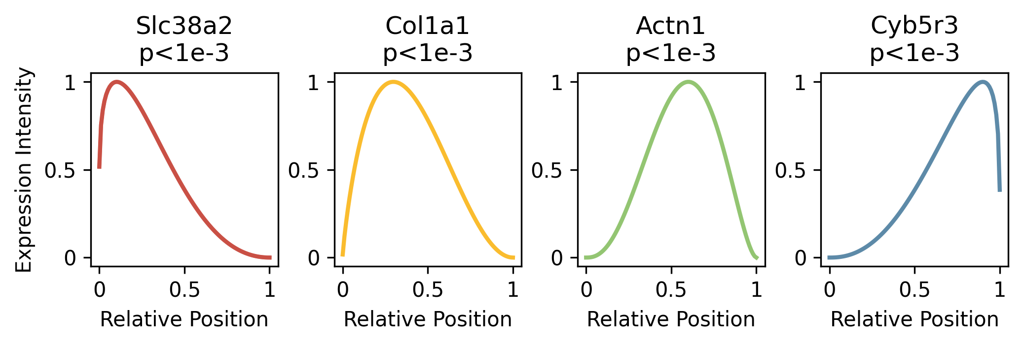
Here Slc38a2 looks like a nuclear localized gene as its estimated expression intensity is high when the relative position is near zero (corresponding to nuclear center); Col1a1 could be a nuclear edge localized gene as its expression intensity peaks around relative position 0.3; Actn1 should be a cytoplasmic localized gene as its expression intensity peaks around 0.6; and Cyb5r3 should be a cell membrane localized gene as its expression intensity peaks near 1 (corresponding to the cell membrane).
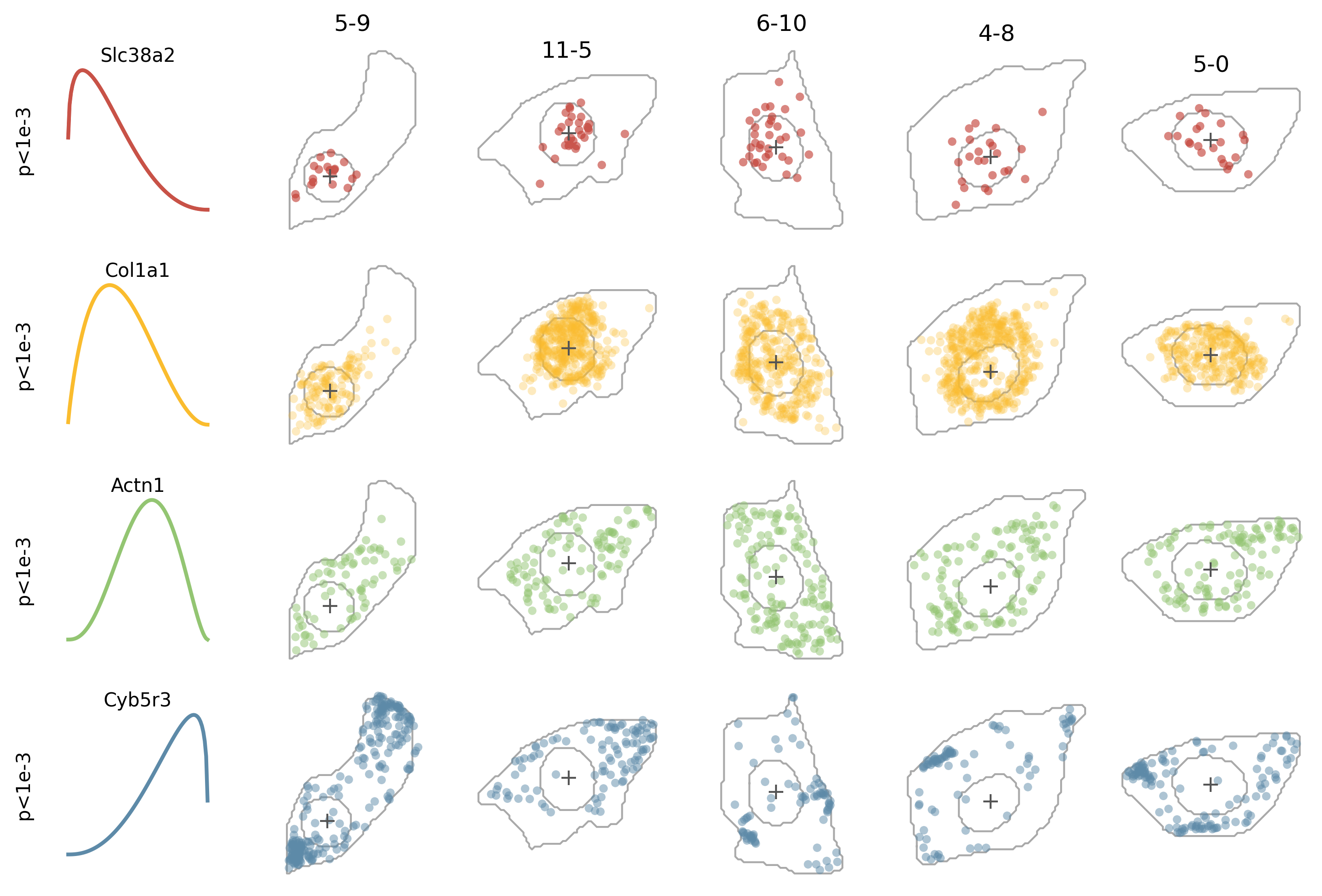
More to plot: We can further plot the cells and genes to have a more intuitive sense of the localization patterns.
alphas = [0.6, 0.3, 0.5, 0.5]

nr = len(genes)
nc = len(cells)+1
ss_nr = 2
ss_nc = 2
fig = plt.figure(figsize=(nc*ss_nc, nr*ss_nr), dpi=300)
gs = fig.add_gridspec(nr, nc,
                      width_ratios=[1]*nc,
                      height_ratios=[1]*nr)
gs.update(wspace=0.1, hspace=0.1)

# plot estimated expression intensities
for j, g in enumerate(genes):
    ax = plt.subplot(gs[j,0])
    pv_g = pv[j]
    lam_g = lam[j]
    lam_g_std = (lam_g-np.min(lam_g))/(np.max(lam_g)-np.min(lam_g))
    ax.plot(np.linspace(0,1,len(lam_g_std)), lam_g_std, lw=2, color=colors[j])
    ax.set_xlim((-0.2, 1.2))
    ax.set_ylim((-0.2, 1.2))
    ax.set_xticks([])
    ax.set_yticks([])
    ax.set_xlabel('')
    ax.text(0.5, 1.1, g, ha='center', va='center')
    if pv_g < 1e-3:
        ax.set_ylabel('p<1e-3')
    else:
        ax.set_ylabel(f'p={pv_g:.3f}')
    ax.spines['top'].set_visible(False)
    ax.spines['right'].set_visible(False)
    ax.spines['left'].set_visible(False)
    ax.spines['bottom'].set_visible(False)

# plot cells and genes
for i, c in enumerate(cells):
    for j, g in enumerate(genes):
        ax = plt.subplot(gs[j,i+1])

        cell_seg_c = cell_seg[cell_seg.cell==c]
        nucleus_seg_c = nucleus_seg[nucleus_seg.cell==c]
        expr_c = expr[expr.cell==c]

        # cell segmentation
        x_reduced = (cell_seg_c.x.values//10) * 10 # reduce resolution to speedup alphashape
        y_reduced = (cell_seg_c.y.values//10) * 10
        points = np.stack((x_reduced, y_reduced)).transpose()
        unique_points = np.unique(points, axis=0)
        alpha_shape_ = alphashape.alphashape(unique_points, 0.1)
        cb_x_, cb_y_ = alpha_shape_.exterior.xy
        ax.plot(cb_x_, cb_y_,
                alpha=0.5,
                color=darkgray, lw=1, zorder=1)

        # nuclear segmentation
        x_reduced = (nucleus_seg_c.x.values//10) * 10 # reduce res to speedup alphashape
        y_reduced = (nucleus_seg_c.y.values//10) * 10
        points = np.stack((x_reduced, y_reduced)).transpose()
        unique_points = np.unique(points, axis=0)
        alpha_shape_ = alphashape.alphashape(unique_points, 0.1)
        cb_x_, cb_y_ = alpha_shape_.exterior.xy
        ax.plot(cb_x_, cb_y_,
                alpha=0.5,
                color=darkgray, lw=1, zorder=1)

        # gene expr
        expr_c_g = expr_c[expr_c.gene==g]
        ax.scatter(expr_c_g.x,
                   expr_c_g.y,
                   s = 20,
                   edgecolor='none',
                   color=colors[j],
                   alpha=alphas[j],
                   zorder=2)

        # cell center
        xc = expr_c.centerX.iloc[0]
        yc = expr_c.centerY.iloc[0]
        ax.scatter(xc, yc, c=darkgray, marker='+',lw=1, s=60, zorder=3)

        ax.set_aspect('equal', adjustable='box')
        #ax.axis('off')
        ax.spines['top'].set_visible(False)
        ax.spines['right'].set_visible(False)
        ax.spines['left'].set_visible(False)
        ax.spines['bottom'].set_visible(False)
        ax.set_xticks([])
        ax.set_yticks([])

        if j==0:
            ax.set_title(c)
        if i==0:
            ax.set_ylabel(g)