A Complete Demo

Here’s a demo introducing a relatively complete ELLA analysis pipeline.

The script and data that will be used in this demo should have already been downloaded (while cloning the ELLA repo). You should be able to find these at your local ELLA folder:

ELLA/scripts/demo/complete_demo/
├── input
│   └── complete_demo_data.pkl
├── output
│   ├── df_nhpp_prepared_saved.pkl
│   ├── df_registered_saved.pkl
│   ├── lam_est.pkl
│   ├── nhpp_fit_results_saved.pkl
│   └── pv_est.pkl
└── complete_demo.ipynb

The data is a subset of the processed seqFISH+ embryonic fibroblast dataset. The input data (input/complete_demo_data.pkl) mainly contains a dictionary of three dataframes corresponding to gene expression, cell segmentation, and nucleus segmentation (optional) with 20 cells and 50 genes.

The script of this demo is complete_demo.ipynb, you should be able to run it locally by yourself (run time around 3min), expecting the following steps and outputs:

1. Initiating ELLA:

   # import ELLA
   from ELLA.ELLA import model_beta, model_null, loss_ll, ELLA
   ella_demo = ELLA(dataset='demo2')
   # load data
   ella_demo.load_data(data_path='input/complete_demo_data.pkl')
   

2. Run the data pre-processing and model fitting steps:

   # register cells
   ella_demo.register_cells()
   # prepare data for model fitting
   ella_demo.nhpp_prepare() 
   # model fitting
   ella_demo.nhpp_fit()
   

   As this could take a couple of minutes, to save time, let’s instead use the saved results in the output folder. ELLA can easily load saved results with:

   # load registered cells
   ella_demo.load_registered_cells(path='output/df_registered_saved.pkl')
   # load prepared data for model fitting
   ella_demo.load_nhpp_prepared(path='output/df_nhpp_prepared_saved.pkl')
   # load model fitting results
   ella_demo.load_nhpp_fit_results(path='output/nhpp_fit_results_saved.pkl')
   

3. Let’s then run the testing and estimation:

   # expression intensity estimation
   ella_demo.weighted_density_est()
   # likelihood ratio test
   ella_demo.compute_pv()
   

4. We can now cluster the estimated (significant) expression intensities into clusters of patterns. We find the optimal number of kmeans clusters K with the ELBOW method where K is chosen as a point where the distortion/inertia begins to decrease more slowly:

   ella_demo.pattern_clustering()
   

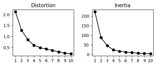
Based on the plots, it seems 5 can be a proper choice, thus let’s proceed with K=5 to obtain 5 pattern clusters:

ella_demo.pattern_labeling(K=5)

Prints:

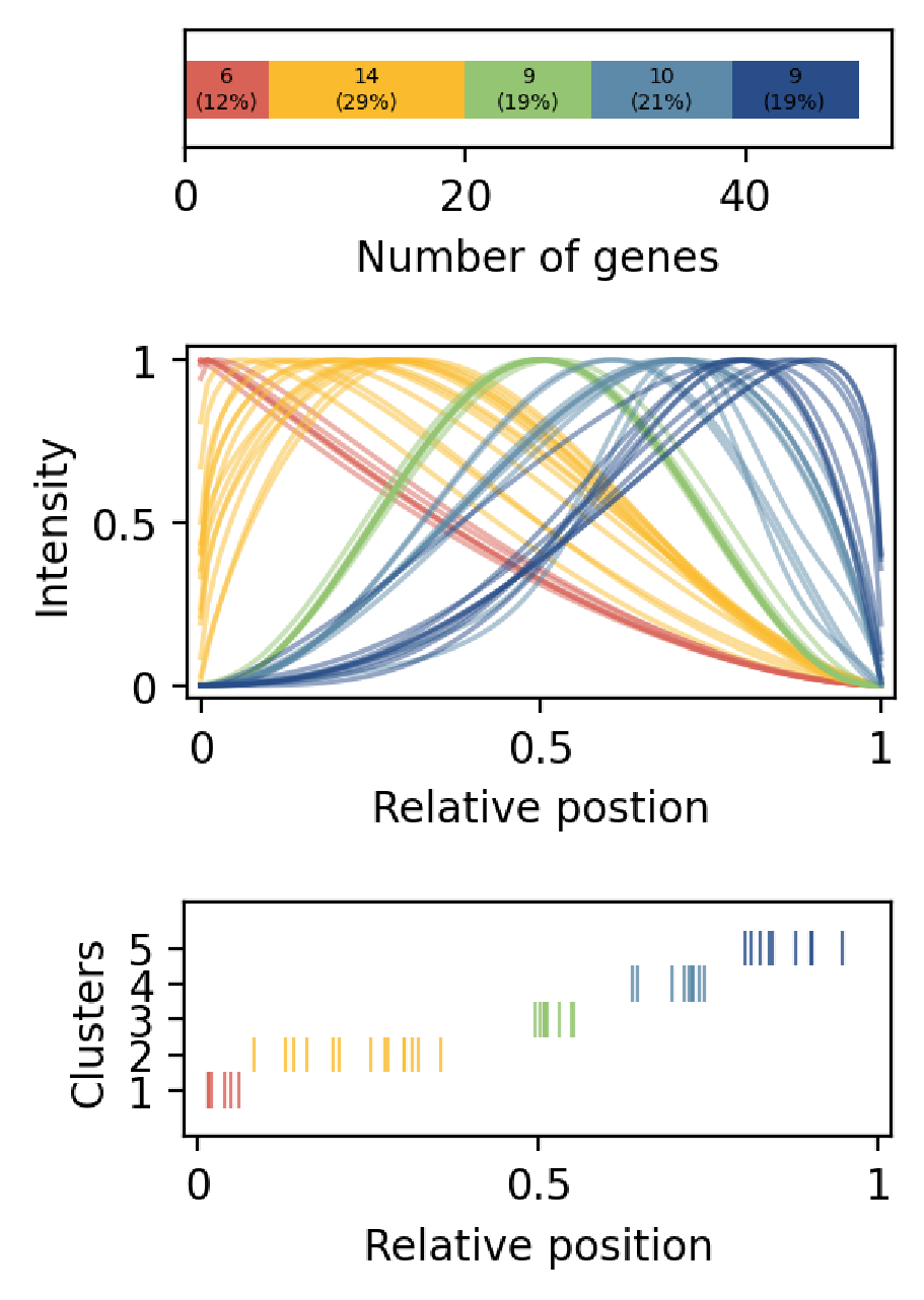
Pattern 1: 6 genes
Pattern 2: 14 genes
Pattern 3: 9 genes
Pattern 4: 10 genes
Pattern 5: 9 genes

Plots: numbers and proportions of significant genes, estimated expression patterns, and estimated pattern scores

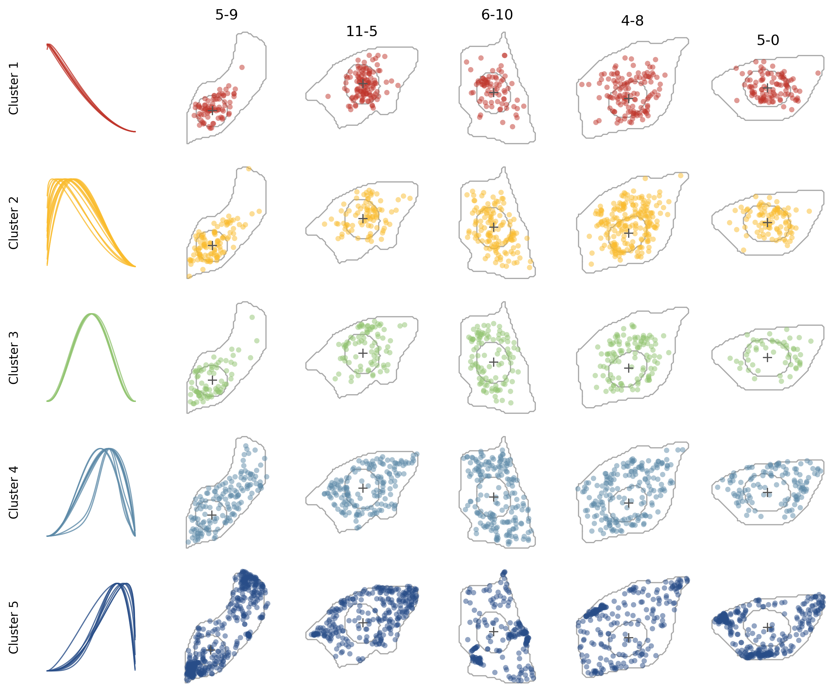
We can overlay all genes in the same cluster in cells to have a more intuitive sense of the patterns.