Inputs

ELLA takes a dictionary of inputs. The two main pieces are a gene expression table (expr) and the cell boundary polygons (cell_poly).

1. Gene expression with nuclear center
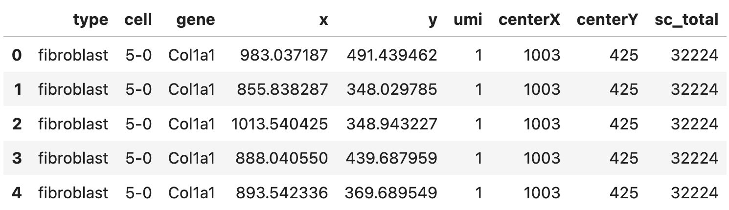
A pandas data frame (expr) with a few columns:

• spatial gene expression including the coordinates (x, y) and the corresponding counts (umi)
• cell center (centerX, centerY)
• cell type (type), cell ID (cell), gene ID (gene)
  
• and the total number expression counts of cells (sc_total), rows corresponding to the same cell should have the same value for this column.

Here’s how the data frame looks like:

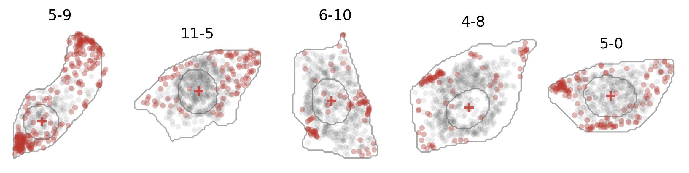
And here’s how the expression of one gene (dots in red) and the cell center (crosses in red) looks like:

2. Cell boundary polygons
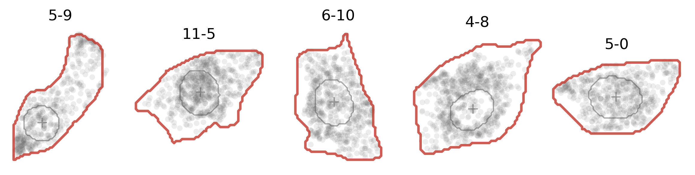
A dictionary (cell_poly) mapping each cell ID to its boundary polygon: an (M, 2) array of (x, y) vertices in the native coordinate frame. ELLA registers each cell to the unit disk by ray-casting against this polygon, so a polygon is required for every cell.

Here’s how the cell boundary looks (in red solid line):

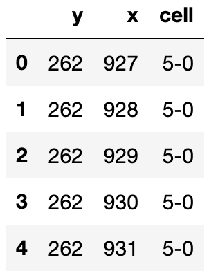
A raster cell segmentation point cloud (cell_seg: a data frame of boundary (cell, x, y) points) is optional and used only for visualization, for example drawing the outlines in the demos; ELLA itself no longer consumes it. It looks like:

Nucleus segmentation
[Optional, for visualization purpose ONLY]

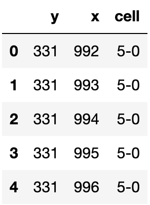
A pands dataframe (nucleus_seg) with 3 columns:

• cell ID (cell)
• the coordinates of points that characterize the nucleus segmentation boundary (nucleus_seg).
  

Here’s how the data frame looks like:

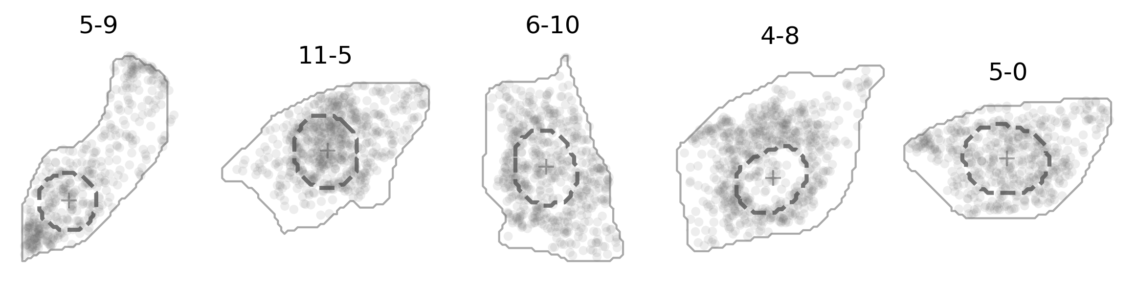
And here’s how it actually looks like (in darkgray dashed line):

Other required inputs

• types a list corresponding to all cell types.
• cells a dictionary of lists corresponding to list of cells in each cell type.
• cells_all a list of all cells across cell types.
• genes a dictionary of lists corresponding to list of genes in each cell type.

How about tweak your own data into the format that ELLA takes and have a try!

Outputs

Running the pipeline (register_cells → nhpp_prepare → nhpp_fit → weighted_density_est → compute_pv, and optionally pattern_clustering → pattern_labeling) stores the results on the ELLA object as dictionaries keyed by cell type. The main ones (these are what the demos read):

• Significance (pv_fdr_tl[type]): per-gene FDR-adjusted p-values (Benjamini-Yekutieli). A gene is significant at sig_cutoff (default 0.05), meaning it has a non-uniform subcellular localization pattern. The pre-adjustment p-values are also kept: pv_cauchy_tl (Cauchy-combined across the 22 kernels) and pv_raw_tl (per-kernel), with the likelihood-ratio test statistics in ts_tl.
• Estimated intensity (weighted_lam_est[type]): per gene, the model-averaged expression-intensity curve as a function of relative position (0 = nuclear center, 1 = cell membrane), evaluated on a length-100 grid. This is the curve the demos plot.
• Peak score (scores[type]): per gene, the relative position where the estimated intensity peaks, a scalar summary of where expression concentrates.
• Pattern clusters (labels_dict[type]): after pattern_labeling(K), the k-means cluster label per gene, with clusters ordered by peak position; non-significant genes are left unlabeled.

Lower-level fit results are available too: the fitted parameters and max log-likelihood per gene and kernel (A_est, B_est, mll_est), the model-averaging weights (weight_ml), and the best kernel per gene (best_kernel_tl).

Each stage also writes a pickle to output/, so results can be reloaded without refitting:

file	written by	contents
df_registered.pkl	register_cells	cells registered to the unit disk
df_nhpp_prepared.pkl	nhpp_prepare	per-gene data prepared for fitting
nhpp_fit_results.pkl	nhpp_fit	fitted A_est, B_est, mll_est
lam_est.pkl	weighted_density_est	scores, weights, weighted_lam
pv_est.pkl	compute_pv	FDR-adjusted p-values

See A Complete Demo for how these outputs are produced and used end-to-end.